Introduction

I am a bit obsessed with drones (UAVs) - for me they offer a world of possibilities for environmental scientists and ecologists. They can be relatively inexpensive and I think there is untapped potential in using the imagery in field survey and assessment. There are also lots of open source tools for working with UAV imagery, so if you can find the money for a drone, you can cheaply and fairly easily process the data and start making use of it.

One of the things I am interested in with UAV imagery is using it to carry out monitoring of habitat creation or restoration. Is it possible to pick up variation in a site, such as where there are more diverse patches of grassland in a field? Is it possible to assess the condition of site and to measure this over time to see if it is getting better? Or conversely to find out that is is getting worse and intervene? There is still no substitute for a trained field surveyor to go our can carry out a survey. But can we get at some of the same information more quickly using a UAV? IF we can, we might be able to rapidly assess a site with a UAV and back up these data with field-based observations less frequently.

UAV imagery

Nearly every UAV you can buy comes equipped with a colour camera. The spec on these varies greatly depending on how much money you are willing to spend. However, using an app (e.g. Dronedeploy, pix4d) you can set up a survey pattern for a site and take overlapping colour images. These images are saved on a SD card as individual files and to make them useable, you need to ‘stitch’ them together. I have had a lot of success using OpenDroneMap - free open source software for stitching together images, plus a whole lot more. You need a fair amount of RAM to do this, but the results are very good. There are of course proprietary products for doing this, but OpenDroneMap does the job without the hefty price tag.

Vegetation idices

However, what the proprietary products do provide are additional outputs beyond the orthomoasic tifs DSM and others. They also enable a user to apply vegetation indices to their images. ODM does not have this functionality, but it is relatively straight forward to apply these indices to your imagery in R.

There are a number of vegetation indices, the most well know of which is Normalised Vegetation Difference Index (NDVI). NDVI requires near-infrared imagery, which is not standard on most domestic UAVs. However there are many others that can be applied to colour (RGB) imagery.

The purpose of this post then is to demonstrate how to apply some of these indices to RGB imagery from a drone.

Loading the UAV image

The image I am using has been ‘stitched’ in OpenDroneMap. It is of a small Local Nature Reserve near my house. The imagery was acquired in September 2019 after a long hot summer, so it was very dry and brown. Consequently this is not the best example for these indices. Nonetheless, it is possible to demonstrate the process, even if the results are not very useful. It would be better to carry out the UAV survey at a time when the vegetation was lush and green.

Firstly, we load the libraries we need:

library(raster)

and then read in the image file stitched together using OpenDroneMap:

img <- raster("image.tif")
plot(img)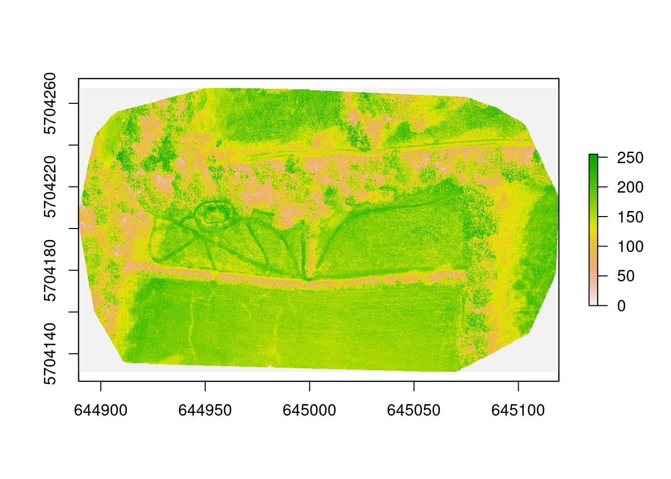

This shows a false colour image of the site. To show the colour image (and to calculate the indices) we need to read each band in separately:

# read in each band separately and then combine into rgb stack
imgR <- raster("image.tif", band = 1)
imgG <- raster("image.tif", band = 2)
imgB <- raster("image.tif", band = 3)

imgRGB <- stack(imgR, imgG, imgB)
plotRGB(imgRGB, 1,2,3)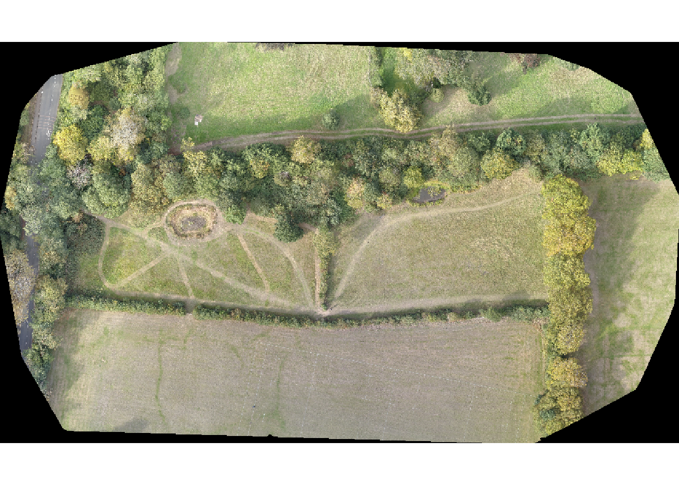

So now we have a colour image of the site. Calculating the various indices requires some raster maths. Some of the available indices can be found in this paper on UAV imagery for monitoring vegetation by Zhang et al. (2019) and I am going to demonstrate two here: Normalised Difference Index (NDI) and the Excessive Green Index (ExG). I have used and adapted code from a notebook on image segmentation by Ivan Lizarazo.

Lizarazo has already coded the ExG index as a function and, using his code as a guide, I have coded a function for the NDI index:

# excess green index
exg <- function(img, r, g, b) {
  r <- img[[r]]
  g <- img[[g]]
  b <- img[[b]]
  vi <- (2 * g - r - b) / (g + r + b)
  return(vi)
}

# normalised difference index
ndi <- function(img, r, g, b) {
  r <- img[[r]]
  g <- img[[g]]
  b <- img[[b]]
  vi <- (g - r)/(g + r)
  return(vi)
}

Oddly, the equation for the Excessive Green Index in Zhang et al. (2019) is different to that in Lizarazo’s paper. I have stuck with Lizarazo’s code, but it is worth investigating what the difference is between the two versions. I am tempted to go with the version in Zhang et al. (2019) as at least there is a literature reference associated with it. For now we press on!

So now I have the functions, I can run my image through them. First, NDI:

img_ndi <- ndi(imgRGB, 1, 2, 3)
plot(img_ndi)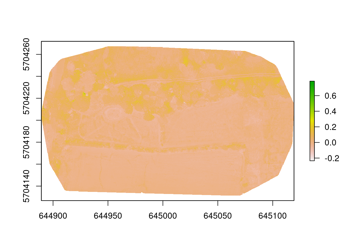

Second, ExG:

img_exg <- exg(imgRGB, 1, 2, 3)
plot(img_exg)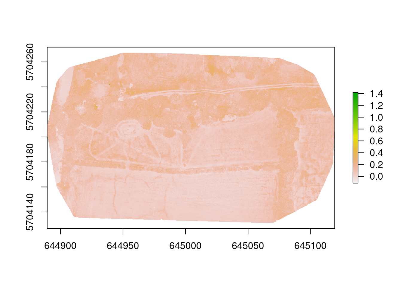

Two indices generated - what can we tell? Well, it was very dry! The trees and hedges are the greenest things on the site and that is shown by the indices. They have the darkest colours (highest values) on both images. We can also clearly see the mown grass paths - these are the lighter lines in the images. The pond in the left field is also highlighted, which was almost dry, but still contained some moisture in the bottom. There also seem to be some darker patches in the right meadow, but it is not clear what they are.

So there is some useful information to be derived from these indices and others may yield more useful data. But it gives a hint to what might be possible.

Next steps

They key thing will be to acquire imagery of a site much earlier in the season (say June) when the vegetation should not be so parched. Hopefully patterns within the vegetation would be clearer. A site with a bit more variation may also reveal clearer patterns.

For monitoring, a good baseline with detailed survey information will be essential. That way you know what you are looking for before you start. UAV imagery and vegetation indices may be sufficient to keep a check on how a habitat is developing over time, punctuated by field survey every 5 years or so. This is what I hope to test over the next year or two.

Code is available on GitHub

Session Info

sessionInfo()

## R version 3.6.3 (2020-02-29)
## Platform: x86_64-pc-linux-gnu (64-bit)
## Running under: Ubuntu 20.04 LTS
## 
## Matrix products: default
## BLAS:   /usr/lib/x86_64-linux-gnu/blas/libblas.so.3.9.0
## LAPACK: /usr/lib/x86_64-linux-gnu/lapack/liblapack.so.3.9.0
## 
## locale:
##  [1] LC_CTYPE=en_GB.UTF-8       LC_NUMERIC=C              
##  [3] LC_TIME=en_GB.UTF-8        LC_COLLATE=en_GB.UTF-8    
##  [5] LC_MONETARY=en_GB.UTF-8    LC_MESSAGES=en_GB.UTF-8   
##  [7] LC_PAPER=en_GB.UTF-8       LC_NAME=C                 
##  [9] LC_ADDRESS=C               LC_TELEPHONE=C            
## [11] LC_MEASUREMENT=en_GB.UTF-8 LC_IDENTIFICATION=C       
## 
## attached base packages:
## [1] stats     graphics  grDevices utils     datasets  methods   base     
## 
## other attached packages:
## [1] raster_3.3-7 sp_1.4-2    
## 
## loaded via a namespace (and not attached):
##  [1] Rcpp_1.0.4.6     bookdown_0.20    codetools_0.2-16 lattice_0.20-40 
##  [5] digest_0.6.25    grid_3.6.3       magrittr_1.5     evaluate_0.14   
##  [9] blogdown_0.20    rlang_0.4.6      stringi_1.4.6    rmarkdown_2.3   
## [13] rgdal_1.5-12     tools_3.6.3      stringr_1.4.0    xfun_0.15       
## [17] yaml_2.2.1       compiler_3.6.3   htmltools_0.5.0  knitr_1.28