Exploring the benefits of street trees with a Shiny app

We receive an enormous number of benefits from trees. They absorb carbon dioxide and produce oxygen, the remove pollution from the air, slow down the movement of water both cleaning it and preventing flooding. They provide shade and shelter and they can make us feel better just by looking at them. There has be an enormous amount written about trees and their benefits, and in the last couple of years the focus has been on them for their role in addressing the climate crisis: everyone wants to plant trees to absorb carbon dioxide, from governments to local wildlife groups and everyone in between. Even the Queen is getting in on the act!

So trees are good, but I worry that they are a useful distraction for some of the harder decisions that everyone needs to take to address the climate crisis - trees are not THE solution to that. There are also plenty of stories of trees being planted in the wrong places and destroying things of far greater value, such as peat bogs or meadows. However, there is one area where I think there should be greater focus on tree planting, and that is in urban areas. All those benefits I spoke about above can be delivered right where people live, in urban areas, making them cleaner and nicer places to live, work and visit. The global coronavirus pandemic has meant that, in the UK at least, more people are working from home, fewer are commuting to work, people are spending more time in their local areas and in local green spaces. The quality of the environment where they live is much more important top people that it ever was.

So I decided to explore the consequences of planting trees in my street here in Reading, UK, and to create an app to let other people do this too. This post describes both the process of doing that, as well as the decisions I made in doing so.

You can explore the app here, or via the ‘Apps’ page on my website.

A bit about my street

I live on Liverpool Road in Reading, UK. This area of the town is called Newtown as it was the new part of town when it was built, but is was actually constructed in the late 1800’s. It is an area of Victorian terraced housing like that found in many towns up and down the UK that are the result of rapidly expanding industry in the late 1800’s. My house was constructed in 1890. In some ways not much has changed since these houses were constructed, with the exception that most people now own a private car. The streets were not designed to accommodate car parking and therefore the roads become quite narrow between two rows of parked cars. I like living here, there is a sense of community that I am starting to feel I belong to.

There are currently two trees on Liverpool Road, both very close to each other by the junction with another road where there is a bit of space for them. There are of course other trees in peoples gardens, but mostly in the back gardens. One is a Hawthorn (Crategous monogyna) and I am not sure what the other one is, as it was planted fairly recently and I have not yet been able to identify it. This second tree replaced another Hawthorn which did not survive.

Car parking

Planting new trees requires space. The pavements are narrow and even a small tree would create a barrier, so they cannot be planted there. This leaves the carriageway, which as I mentioned, is largely taken up with car parking and a single one way passage between them. This means that planting trees in the carriageway (in a tree pit of course, not just hacking a hole out of the tarmac!) will reduce the parking capacity on the street.

In order to account for this in my analysis, I counted the number of cars parked on the street and the number of spaces in which a car could be parked. I only did this once, so it is a very crude estimate. On the 16th November 2020 there were 144 cars parked on the road and an additional 28 spaces which could fit cars, meaning total car parking capacity for 173 spaces. It is important to note that there are not parking bays marked out on the street, meaning that the parking is not very efficient. I hypothesise that by marking out bays, the parking capacity would be increased.

To estimate the potential parking capacity created from marking bays, I measured the amount of parking space in Liverpool Road from OpenStreetMap data and aerial imagery in QGIS. I estimate that there is 995 metres of parking space on Liverpool Road. This measurement won’t be as accurate as getting out there with a tape measure, but I do not have a tape measure long enough for that! According to Bracknell Forest Council’s parking standard a parking space should be 4.8 metres long. If we are generous and allow 5 metres for a car parking space, the Liverpool Road has capacity for 199 spaces. In theory then, just by marking out parking bays, it would be possible to increase parking capacity by 26 spaces. I am aware that this does not incorporate space for accessible parking spaces, to the real number will be lower.

How many trees?

How many trees could be planted in Liverpool Road? Obviously the more trees the greater the benefits, but also the more parking capacity that would be absorbed. So I decided to test some different scenarios. In my last job I was working on the Oxfordshire Tree and Woodland Project and in their street tree analysis they used a minimum distance of 7 metres between street trees. I am not sure of the origin of this value, but I have stuck with it. Therefore trees would be planted at least 7 metres from another tree on the street. I also used minimum distances of 14 metres and 28 metres to explore how tree density affects both benefits and parking.

I needed to create some trees. To do this I downloaded the OpenStreetMap data for Reading from the Geofabrik downloads page and extracted the line data for the roads. The road lines run down the centre of the roads, so I had to create parallel lines to get the lines at the edge of the road where the trees would be planted. I used the parallel lines buffer tool from the QGIS processing tool box to do this.

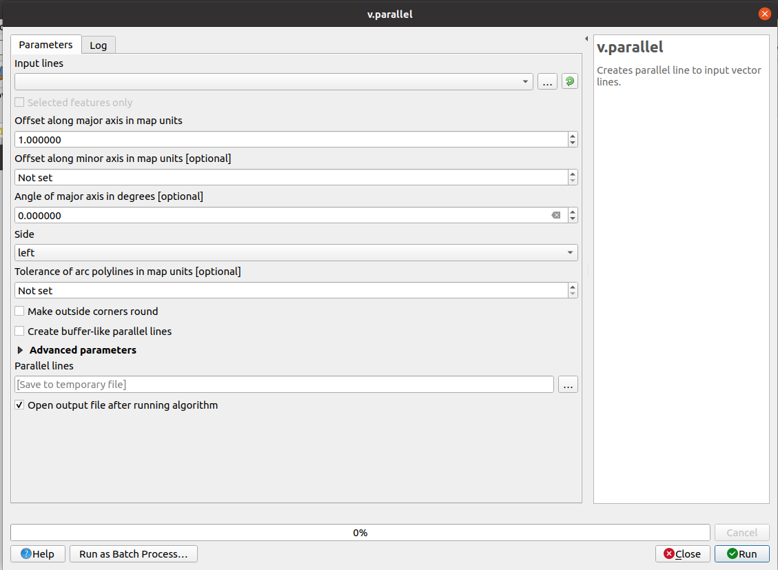
As a quick aside, the search function in the QGIS Processing toolbox is amazing. I did not know if there was a tool to do parallel buffers, but I just types key words into the search box and hey presto, there are two! It is fair to say that is possible to do most things with a QGIS processing tool and the search box helps you find the right one.

Anyway, I now had parallel lines for my road centre line, and I used these lines to create points on for trees. To do this I used the random points along lines tool in QGIS, setting a minimum distance between points and a maximum number of points, calculated from dividing the line lengths by the minimum distance between trees.

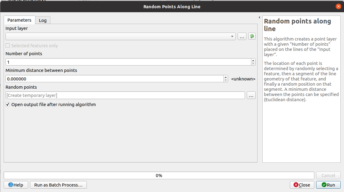
This worked out very well, so I now had three point data sets representing trees at different planting densities. You can find out how many trees this is in the app!

What trees?

Now I knew how many trees could be planted, I needed to decide what sort of trees they were. The Trees and Design Action Group has a guide for the selection of tree species for green infrastructure. I used this guide to select four species of tree that would cope with being planted in streets, that were not too big, and were reasonably resilient to pollution and drought. I chose three UK native species and one European species: Field maple (Acer campestre), Hawthorn (Crategous monogyna), Cherry plum (Prunus cerasifera) and Swedish Whitebeam (Sorbus intermedia). I wanted to pick mostly native species as they would have a value for biodiversity, as well as providing benefits to residents of Liverpool Road. There are plenty of alternatives that could have been picked, each with their own pros and cons, but this is as good a species mix as any.

I needed to assign these tree species to the points I had created and to do this I found a neat trick in R:

df %>% 
  group_by(grp) %>% 
  mutate(var_n = sample(var, size = n(), prob = probs, replace = TRUE))

where probs is a vector of probabilities:

probs <- c(0.30, 0.15, 0.30, 0.25)

I decided that the proportions of each species should be as follows:

• Acer campestre - 30%
• Crategous monogyna - 15%
• Prunus cerasifera - 30%
• Sorbus intermedia - 25%

This mix prioritised shorter trees over taller trees. I also set the diameter at breast height (DBH) to 9 cm for all the trees, deciding that this was a sensible size tree to be planting.

In planting the trees I assumed they would be planted in tree pits that are 1.2 metres by 1.2 metres. Proper tree advice is of course required!

Calculating the benefits

At this point I had decided how many trees I was proposing to plant, of which species and of what size. What I needed to now do was calculate the benefits these trees would provide. To do this I used the i-Tree Eco tool. This tool has been developed by the USDA Forest Service, the Davey Tree Expert Company and others to calculate the ecosystem service benefits of trees. The Eco tool is just one among a suite of tools for doing this and much more. It is a powerful tool for doing this, but in its simplest form, all it requires is the species of tree and its DBH.

The app

The app itself is a fairly simple Shiny app. I have used the {shinydashboard} package for the main components, but there is only one tab, so it was not strictly necessary. However, I think it looks slightly nicer than a vanilla shiny app.

The app uses a single csv file with all of the data in it. There is a dropdown menu to select the distance between trees and then there is a map and some value boxes which update with the data. A map shows the indicative position of the trees and is colour coded by species. That proved to be a bit tricky, so I will explore that a bit further here. I had to create a palette for the species in the csv as follows:

pal <- colorFactor(topo.colors(4), street_trees$Species)

This essentially assigns a color to each species in the csv file. I was then able to pass this palette as an argument to both the markers and the legend like so:

leaflet(st()) %>%
            addTiles() %>%
            setView(-0.94680369, 51.456922, zoom = 16) %>%
            addCircleMarkers(lat = ~y, lng = ~x, radius = 1, color = ~pal(Species)) %>% 
           addLegend(position = "topright", pal = pal, values = st()$Species, title = "Tree species")

In an earlier version of the app I had a table with the values for carbon and pollution in it, but it didn’t look that good. So I decided to use value boxes to display these values instead. I think these better communicate the different values than a table, but others might find a table more useful. To update these value boxes there are two bits of reactive code required to respond to a change int he selection from the dropdown menu. The first is to filter the csv data to those trees with ‘centres’ (i.e. distances between trees) that meet the dropdown value. The second was to calculate the car parking spaces. For both of these I used the eventReactive() function, as in the following example:

sts <- eventReactive(input$centre, {
        filter(street_trees, centres == input$centre) %>%
            summarise(`Carbon stored (kg)` = sum(Carbon_Storage_kg),
                      `Carbon Sequestered (kg/yr)` = sum(Carbon_Sequestration_kg_yr),
                      `Pollution Removed (g/yr)` = sum(Pollution_Removal_g_yr))

This bit of code also calculates the total values for the value boxes. And that is it really. The value boxes were fun to produce, deciding on colours and trying to find suitable icons for them. I’m not entirely happy with the icons I have used, but they were the best ones I could find. I didn’t spend a lot of time on this, so there may be better options in a different icon library.

Deploying the app

To deploy the app I am using the DigitalOcean app platform. I have written a bit about this before, but I have learned a bit more about deploying apps using this since then, so here I will describe what I did this time.

The main thing that is required for deploying a Shiny app on DO is a Dockerfile. DO essentially creates a Docker container to serve the app in. Fortunately the amazing Rocker project has done a lot of the hard work for R folk by providing images for common R applications. I was able to use one of their images for Shiny to base my own image on. A Dockerfile is essentially a set of instructions for how to build an image which has all of the things that you need for running a Shiny app - an operating system, some system libraries, some R packages, Shiny server and of course your app. The Dockerfile looks like this:

# Base image https://hub.docker.com/u/rocker/
FROM rocker/shiny:latest

# system libraries of general use
## install debian packages
RUN apt-get update -qq && apt-get -y --no-install-recommends install \
    libxml2-dev \
    libcairo2-dev \
    libsqlite3-dev \
    libmariadbd-dev \
    libpq-dev \
    libssh2-1-dev \
    unixodbc-dev \
    libcurl4-openssl-dev \
    libssl-dev

## update system libraries
RUN apt-get update && \
    apt-get upgrade -y && \
    apt-get clean

# install R packages
RUN R -e "install.packages('shinydashboard')"

RUN R -e "install.packages(c('leaflet', 'readr', 'dplyr', 'DT'), dependencies=TRUE, repos='http://cran.rstudio.com/')"

# copy necessary files
## app folder
COPY app.R /srv/shiny-server/street_trees/
COPY street_trees.csv /srv/shiny-server/street_trees/

RUN sudo rm /srv/shiny-server/index.html
COPY index.html /srv/shiny-server/index.html
COPY /index_files /srv/shiny-server/index_files/
COPY dc_temp.jpg /srv/shiny-server/dc_temp.jpg

The first line grabs the Shiny image from Rocker. Then there is some standard Linux command line stuff to install and update the libraries for the OS (in this case Debian). Next comes the commands to install R packages to make them available inside the container. For some reason, the {shinydashboard} package would not install as part of the second line of install code and I do not know why. It installed fine when I did it on its own!

Next you have to copy your app into the shinyserver file directory. Shinyserver is rather clever as if there is an app in the directory, it will serve it, no questions asked. I added the app into a folder all of its own, along with the csv file that is read in by the app. This means when you go to the app.URL/street_trees/ the app will be waiting there for you.

The final bit of the Dockerfile is about replacing the standard shinyserver landing page with one I created myself.

---
title: "Hello, I'm Dan Carpenter"
image: "dc_temp.jpg"
# links:
#   - LinkedIn: "https://www.linkedin.com/in/dan-carpenter-cenv-057b512a/"
#   - Twitter: "https://twitter.com/drdcarpenter"
#   - GitHub: "https://github.com/drdcarpenter"
output:
  postcards::trestles
---
 
## My Apps

Here are some apps I have made using Shiny and R.

<link rel="stylesheet" href="https://cdnjs.cloudflare.com/ajax/libs/font-awesome/4.7.0/css/font-awesome.min.css">
<style>
.btn {
  background-color: DarkGrey;
  border: none;
  color: white;
  padding: 12px 16px;
  text decoration: none;
  font-size: 16px;
  cursor: pointer;
}

/* Darker background on mouse-over */
.btn:hover {
  background-color: Green;
}

.button2 {border-radius: 4px;}

</style>

<table style="width:100%">
  <tr>
    <td><a href="/street_trees/" target="_blank"><button class="btn button2"><i class="fa fa-tree"></i> Street Trees app</button></a></td>
    <td>A Shiny application to explore the benefits we gain from street tree planting.</td>
  </tr>
</table>

Code

All of the code for the app, the Dockerfile and the postcards Rmd is on Github and you can access the app via the ‘App’ menu at the top of my website.

Feedback

I would be very pleased to receive feedback on the app and the general idea of additional street trees and the benefits they could provide. There is currently a funding drive for more trees in Reading, but I am not sure if anyone has decided where these trees will go. I hope it is not on existing green space of value and I would like to think one of the aims of this tree planting is to improve the environment of residents in Reading. We will see! Anyway, you can get in touch via Twitter, LinkedIn or email - all the details are on my website.

Session Info

## R version 3.6.3 (2020-02-29)
## Platform: x86_64-pc-linux-gnu (64-bit)
## Running under: Ubuntu 20.04.1 LTS
## 
## Matrix products: default
## BLAS:   /usr/lib/x86_64-linux-gnu/blas/libblas.so.3.9.0
## LAPACK: /usr/lib/x86_64-linux-gnu/lapack/liblapack.so.3.9.0
## 
## locale:
##  [1] LC_CTYPE=en_GB.UTF-8       LC_NUMERIC=C              
##  [3] LC_TIME=en_GB.UTF-8        LC_COLLATE=en_GB.UTF-8    
##  [5] LC_MONETARY=en_GB.UTF-8    LC_MESSAGES=en_GB.UTF-8   
##  [7] LC_PAPER=en_GB.UTF-8       LC_NAME=C                 
##  [9] LC_ADDRESS=C               LC_TELEPHONE=C            
## [11] LC_MEASUREMENT=en_GB.UTF-8 LC_IDENTIFICATION=C       
## 
## attached base packages:
## [1] stats     graphics  grDevices utils     datasets  methods   base     
## 
## loaded via a namespace (and not attached):
##  [1] compiler_3.6.3  magrittr_2.0.1  bookdown_0.20   tools_3.6.3    
##  [5] htmltools_0.5.0 yaml_2.2.1      stringi_1.4.6   rmarkdown_2.5  
##  [9] blogdown_0.20   knitr_1.30      stringr_1.4.0   digest_0.6.27  
## [13] xfun_0.19       rlang_0.4.9     evaluate_0.14