Palmer Park leisure centre and biodiversity net gain
Introduction
Palmer Park is in the Park ward of east Reading (UK). It has a leisure centre among its facilities and there is a planning proposal to extend this centre to create a swimming pool. East Reading used to have a swimming pool at Arthur Hill - a Victorian baths which Reading Borough Council sold and is now being turned into housing. The leisure centre extension is the Council’s proposal to provide a new swimming pool in east Reading, as well as other new facilities.
This post details my assessment of the application and its ability to deliver a biodiversity net gain in accordance with the National Planning Policy Framework. It is also an opportunity to develop some R code to process the biodiversity metric which is key to calculating net gain. I have included my code here should it help others. I intend to do further work on this code to create functions that produce the summary tables in this document and perhaps wrap it all into a package. In the meantime the code is here for anyone to use, as well as being on Github.
I do this stuff in my day job, so I have a lot of experience in biodiversity net gain - it is in my job title. I also help teach other UK ecologists (and some from elsewhere in Europe) how to use the biodiversity metric for the Chartered Institute of Ecology and Environmental Management. However, what follows is merely my professional opinion and is not definitive.
The application itself does not include an assessment of biodiversity net gain, despite biodiversity net gain being a requirement of both national and local planning policy, as I set out below. Why this is, I do not know.
Biodiversity net gain
First a little bit about biodiversity net gain - what is it? Simply put it is development that leaves biodiversity in a better state than before. For example, in this case, the leisure centre development must leave biodiversity in a better state than it is now, before the development takes place (assuming it is approved of course). What do we mean by biodiversity? Well in this case it is restricted to habitats, which of course ignores all of the other biodiversity in the world; genes, species and ecosystems. But that is how the metric works.
Planning policy
The National Planning Policy Framework (NPPF) is the document that guides planning in England. In it there are specific references to biodiversity net gain.
Paragraph 170 of the NPPF states:
Planning policies and decisions should contribute to and enhance the natural and local environment by:…
- minimising impacts on and providing net gains for biodiversity, including by establishing coherent ecological networks that are more resilient to current and future pressures;…
Paragraph 174 of the NPPF states:
To protect and enhance biodiversity and geodiversity, plans should:…
- promote the conservation, restoration and enhancement of priority habitats, ecological networks and the protection and recovery of priority species; and identify and pursue opportunities for securing measurable net gains for biodiversity.
The NPPF is very clear, development should provide measurable net gains for biodiversity. The metric (more on that in a minute) provides the means to measure net gain.
Reading Borough Council has a Local Plan adopted in 2019. This sets out local policy for planning. In it there is policy EN12 which says:
- On all sites, development should not result in a net loss of biodiversity and geodiversity, and should provide a net gain for biodiversity wherever possible.
So Reading Borough Council’s Local Plan also says that development should provide a net gain in biodiversity. So let’s see if the leisure centre proposals do!
The metric
I have mentioned this a few times now, but ‘the metric’ is a spreadsheet based calculator for biodiversity net gain assessments. It was put together by Natural England staff and it is free to download from their website. It is currently undergoing a revision, the new version due out in ‘Spring 20201’.
Essentially, the metric works by calculating the difference between the habitats on a site before and after a development to see if there is a net gain. It is a little bit more complicated than that, but that is the basics. It does require a good habitats survey and an assessment of the habitats condition. It also really needs those habitats mapping in GIS or a CAD system to that the areas of the habitats can be accurately calculated.
Here I will run through how I calculated the net change in biodiversity units from the information available on the Reading BC planning portal and some data I created using GIS. It is important to note that the data I am going to run through below is data I have created and may not be an accurate reflection of the exact scheme, but it is the best I can do with the information available. First load the packages and read in the metric data.
library(openxlsx)
library(dplyr)
library(janitor)
library(readr)
library(tibble)

metric <- "Palmer Park Biodiversity Metric 2.0 Calculation Tool Beta Test - December 2019 Update.xlsm"

m <- loadWorkbook(metric)
Baseline habitats
The first thing to do is calculate the baseline habitats for the development site. But before I could do that I have to map the red line boundary - or the boundary of the application site. This was provided as a pdf on the planning portal:
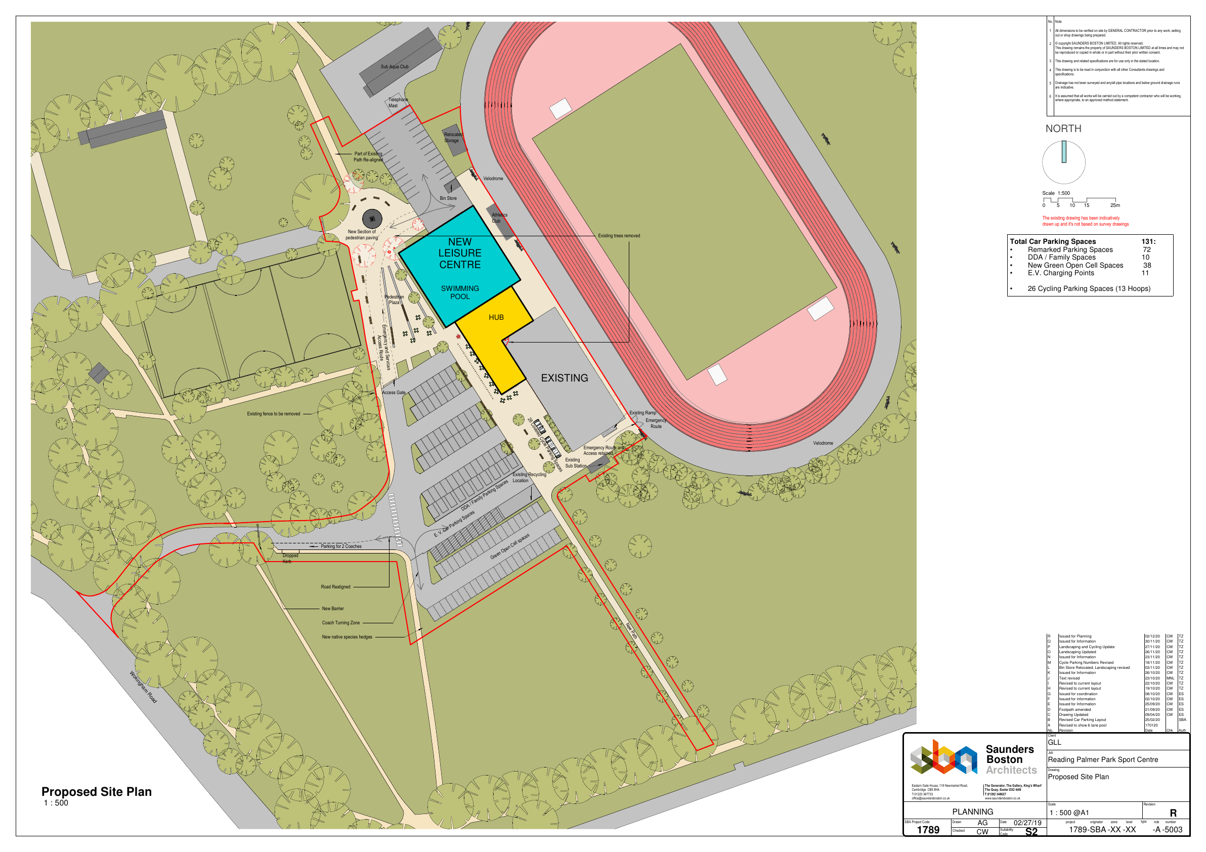
Map showing red line boundary for application site
I had to convert this into a png file so that I could georeference it in QGIS. There is a handy little library in R for doing this: pdftools. The code below shows how to convert a pdf to a png file. I am trying to get this to run as a script in QGIS, but so far I have not had any luck. The first time I tried, QGIS spent hours installing packages, despite many of them already being installed in R. I need to try again.
library(pdftools)

pdf_file <- file.path("mypdf.pdf")
pdf_convert(pdf_file)
Anyway, once I had the image georeferenced, I was able to trace the red line as a vector layer in QGIS. This was then the starting point to map the habitats on the site. There is an ecology report submitted withe application. I know the firm who did it well and they are a good outfit, so I am confident in their assessments. Their maps was not to scale however, so it was not possible to use that to create the habitats data. Instead I used aerial imagery to split up this red line into the different habitats, using the ecology report as a guide for the habitat types.
I now had the different habitat parcels mapped and areas for each of them calculated in QGIS. Here is a map showing those habitats.
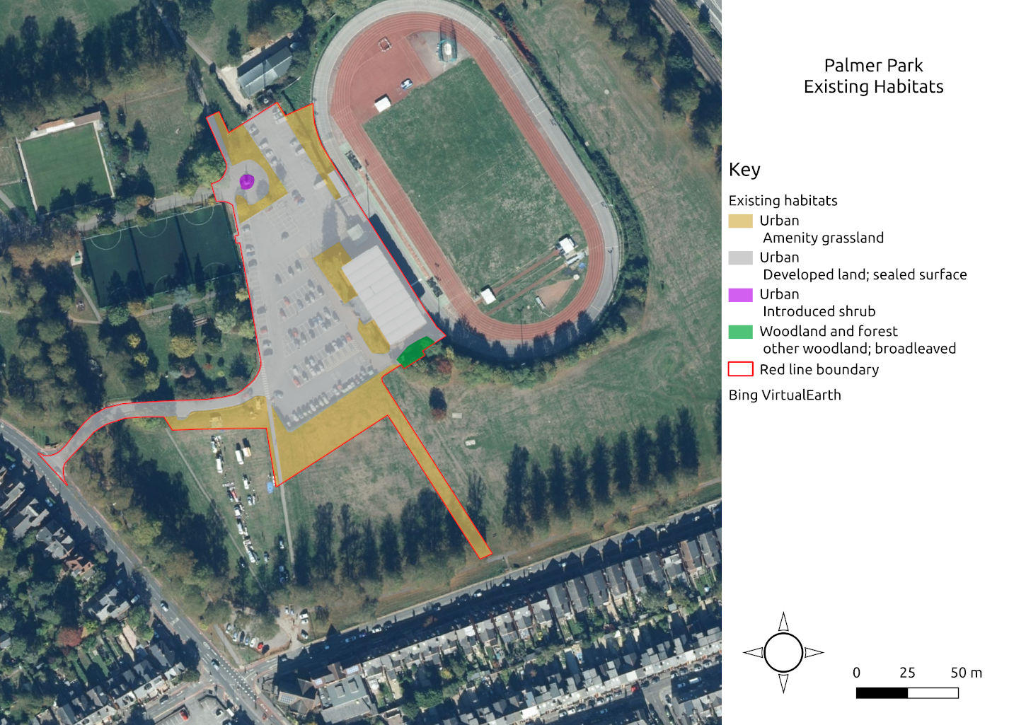
Map of existing habitats on development site
Entering baseline data into the metric
I entered the habitat types and areas into the metric. It automatically applies a ‘distinctiveness’ score - this is a measure of a habitats importance for wildlife. I entered a condition score, following the guidance in the technical document that accompanies the metric. Connectivity scores are a function of distinctiveness - if distinctiveness is ‘Low’ or ‘Medium’ connectivity is ‘Low’. If distinctiveness is ‘High’ or ‘Very High’ then connectivity is ‘Medium’. This rule is set out in the user guide. Strategic significance relates to the importance of a habitat in a particular location. I wrote a little bit about this on LinkedIn. Essentially, if the location of the habitat has been identified as important for nature conservation then it is said to be strategically significant. Palmer Park does not fall into this category and therefore strategic significance is ‘Low’. Entering all of these data into the metric gives you a total unit score for the site. This is summarised in the table below.
baseline <- function(metric){

  b <- read.xlsx(metric, sheet = 9, startRow = 4, skipEmptyRows = TRUE, skipEmptyCols = TRUE) %>%
    select(3:5, 7, 9, 13, 16) %>%
    remove_empty(which = c("rows", "cols")) %>%
    row_to_names(row_number = 2, remove_row = TRUE) %>%
    rename(Habitat = 1, Area = 2, Connectivity = 5, `Biodiversity units` = 7) %>%
    slice(1:4)

  b$Area <-  as.numeric(as.character(b$Area))
  b$`Biodiversity units` <- as.numeric(as.character(b$`Biodiversity units`))

  b <- adorn_totals(b)

  return(b)

}

b <- baseline(m)

knitr::kable(b, digits = 2)| Habitat | Area | Distinctiveness | Condition | Connectivity | Strategic significance | Biodiversity units |
|---|---|---|---|---|---|---|
| Urban - Amenity grassland | 0.38 | Low | Poor | Low | Low Strategic Significance | 0.76 |
| Urban - Introduced shrub | 0.01 | Low | Poor | Low | Low Strategic Significance | 0.02 |
| Urban - Developed land; sealed surface | 0.91 | V.Low | N/A - Other | N/A | Low Strategic Significance | 0.00 |
| Woodland and forest - Other woodland; broadleaved | 0.01 | Medium | Poor | Low | Low Strategic Significance | 0.04 |
| Total | 1.31 | - | - | - | - | 0.82 |
The baseline habitats generate 0.82 biodiversity units.
Retained habitats
Now that the baseline is mapped, the habitats proposed by the development need to be mapped to carry out the net gain calculation. For this I used a plan of the development as submitted with the application, from which I had previously digitised the red line boundary (see the map earlier).
The differences are that some of the amenity grassland is lost to create a larger car park, but some different small areas are created in the new car park. The woodland in the application boundary is also being removed as part of the development proposals. Given the location, I am not sure that all that parking space is necessary - surely we should be encourage to walk, cycle or get the bus to the leisure centre! Anyway, that is editorialising! I was able to map the habitats and calculate the area of each habitat. I assigned future condition appropriately and all of the other parameters remained the same. A map of the proposed habitats is below.
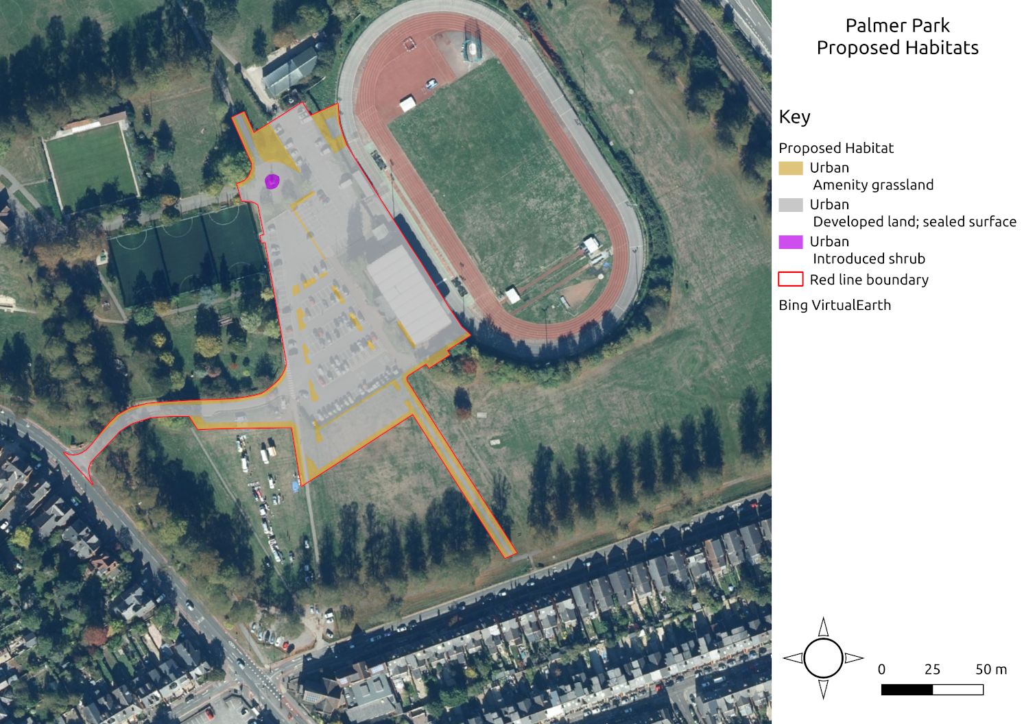
Map of proposed habitats on site
The proposed scheme generates 0.44 biodiversity units, as summarised in the table below. This does not include the area of the land retained by the proposed development.
# create summary table of proposed units
# this only does the created habitats, not the retained or enhanced habitats

proposed <- function(metric){

  p <- read.xlsx(metric, sheet = 10, skipEmptyRows = TRUE, skipEmptyCols = TRUE) %>%
    select(1:3, 5, 7, 11, 17) %>%
    remove_empty(which = c("rows", "cols")) %>%
    row_to_names(row_number = 4, remove_row = TRUE) %>%
    rename(Habitat = 1, Area = 2, Connectivity = 5, `Strategic significance` = 6, `Biodiversity units` = 7) %>%
    slice(2:3)

  p$Area <- as.numeric(as.character(p$Area))
  p$`Biodiversity units` <- as.numeric(as.character(p$`Biodiversity units`))

  return(p)

}

p <- proposed(m)

# retained habitats

r <- read.xlsx(m, sheet = 9, startRow = 4, skipEmptyRows = TRUE, skipEmptyCols = TRUE)
retained <- r %>%
  select(3,17,5,7,10,13,20) %>%
  slice(2:5) %>%
  row_to_names(row_number = 1, remove_row = TRUE) %>%
  rename(Habitat = 1, Area = 2, Connectivity = 5, `Biodiversity units` = 7)

retained$Area <- as.numeric(as.character(retained$Area))
retained$`Biodiversity units` <- as.numeric(as.character(retained$`Biodiversity units`))

# proposed units table

proposed <- bind_rows(retained, p) %>%
  slice(-6) %>%
  adorn_totals()


knitr::kable(proposed, digits = 2, format.args = list(scientific = FALSE))| Habitat | Area | Distinctiveness | Condition | Connectivity | Strategic significance | Biodiversity units |
|---|---|---|---|---|---|---|
| Urban - Amenity grassland | 0.16 | Low | Poor | Unconnected habitat | Low Strategic Significance | 0.32 |
| Urban - Introduced shrub | 0.01 | Low | Poor | Unconnected habitat | Low Strategic Significance | 0.02 |
| Urban - Developed land; sealed surface | 0.91 | V.Low | N/A - Other | Assessment not appropriate | Low Strategic Significance | 0.00 |
| Urban - Amenity grassland | 0.05 | Low | Poor | Low | Low Strategic Significance | 0.10 |
| Urban - Developed land; sealed surface | 0.18 | V.Low | N/A - Other | N/A | Low Strategic Significance | 0.00 |
| Total | 1.31 | - | - | - | - | 0.44 |
Net change in biodiversity
As can be seen from the next table, the scheme does not deliver a net gain in biodiversity. There is a net loss of 0.38 units (or -47%). As such the scheme does not accord with the NPPF or Local Plan policy EN12 and should be rejected.
# results table
results <- read.xlsx(m, sheet = 6, skipEmptyRows = TRUE, skipEmptyCols = TRUE) %>%
  row_to_names(row_number = 1, remove_row = TRUE) %>%
  clean_names() %>%
  rename(`Headline Results` = headline_results," " = na, Units = na_2) %>%
  remove_rownames()

options(knitr.kable.NA = "")

knitr::kable(results, digits = 2, format.args = list(scientific = FALSE, na.encode = TRUE))| Headline Results | Units | |
|---|---|---|
| On-site baseline | Habitat units | 0.82 |
| Hedgerow units | 0.00 | |
| River units | 0.00 | |
| On-site post-intervention | ||
| (Including habitat retention, creation, enhancement & succession) | Habitat units | 0.44 |
| Hedgerow units | 0.00 | |
| River units | 0.00 | |
| Off-site baseline | Habitat units | 0.00 |
| Hedgerow units | 0.00 | |
| River units | 0.00 | |
| Off-site post-intervention | ||
| (Including habitat retention, creation, enhancement & succession) | Habitat units | 0.00 |
| Hedgerow units | 0.00 | |
| River units | 0.00 | |
| Total net unit change | ||
| (including all on-site & off-site habitat retention/creation) | Habitat units | -0.38 |
| Hedgerow units | 0.00 | |
| River units | 0.00 | |
| Total net % change | ||
| (including all on-site & off-site habitat creation + retained habitats) | Habitat units | -0.47 |
| Hedgerow units | 0.00 | |
| River units | 0.00 |
Delivering a net gain for biodiversity
It would be possible to deliver a net gain for biodiversity by enhancing an area of grassland within the park. I have looked at how much land would be required and what the enhancement should be. The metric is designed so that any losses are offset on a ‘like-for-like’ basis - in this case grassland has been lost, so grassland should be created or enhanced. An area of amenity grassland in the wider park of ~0.15 hectares could be enhanced and managed as wildflower grassland. This grassland would generate sufficient biodiversity units to offset the impact of the development. There was also a small area of woodland lost - the park is not the best place to create woodland, but another woodland (such as The Coal woodland) could be enhanced through planting and management to offset the woodland impacts. All this would of course need to be agreed to by Reading Borough Council and a commitment to manage these enhancements for 30 years entered into. The developer would need to fund that management, so this should be perfectly possible (although of course the developer is actually the Council!).
Summary
In summary, both the National Planning Policy Framework and the Reading Local Plan support the delivery of biodiversity net gain for development. The scheme for the leisure centre cannot demonstrate that it can deliver a biodiversity net gain and so should be refused until it can.
All of the data and a copy of the metric for this article can be found on Github, so others are able to check what I have done and update or improve it.
sessionInfo()## R version 3.6.3 (2020-02-29)
## Platform: x86_64-pc-linux-gnu (64-bit)
## Running under: Ubuntu 20.04.1 LTS
##
## Matrix products: default
## BLAS: /usr/lib/x86_64-linux-gnu/blas/libblas.so.3.9.0
## LAPACK: /usr/lib/x86_64-linux-gnu/lapack/liblapack.so.3.9.0
##
## locale:
## [1] LC_CTYPE=en_GB.UTF-8 LC_NUMERIC=C
## [3] LC_TIME=en_GB.UTF-8 LC_COLLATE=en_GB.UTF-8
## [5] LC_MONETARY=en_GB.UTF-8 LC_MESSAGES=en_GB.UTF-8
## [7] LC_PAPER=en_GB.UTF-8 LC_NAME=C
## [9] LC_ADDRESS=C LC_TELEPHONE=C
## [11] LC_MEASUREMENT=en_GB.UTF-8 LC_IDENTIFICATION=C
##
## attached base packages:
## [1] stats graphics grDevices utils datasets methods base
##
## other attached packages:
## [1] tibble_3.0.4 readr_1.3.1 janitor_2.0.1 dplyr_1.0.2 openxlsx_4.2.3
##
## loaded via a namespace (and not attached):
## [1] Rcpp_1.0.5 knitr_1.30 magrittr_2.0.1 hms_0.5.3
## [5] tidyselect_1.1.0 R6_2.4.1 rlang_0.4.9 highr_0.8
## [9] stringr_1.4.0 tools_3.6.3 xfun_0.19 htmltools_0.5.0
## [13] ellipsis_0.3.1 yaml_2.2.1 digest_0.6.27 lifecycle_0.2.0
## [17] crayon_1.3.4 bookdown_0.20 zip_2.1.1 purrr_0.3.4
## [21] vctrs_0.3.6 snakecase_0.11.0 glue_1.4.2 evaluate_0.14
## [25] rmarkdown_2.5 blogdown_0.20 stringi_1.4.6 compiler_3.6.3
## [29] pillar_1.4.7 generics_0.0.2 lubridate_1.7.9 pkgconfig_2.0.3